One of our trainers showed me this function when I was trying to find data in a huge worksheet. It is a fantastic function for List Management and saves me lots of time and stressing.
Here is a simple example to demonstrate how to use filters in Excel.
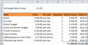
I have my worksheet with details of budgeted items for a business trip. I want to try and identify the one-off items to see if I can reduce those costs.
Here is my worksheet with details of the items and units. I want to filter the results by cost per person.

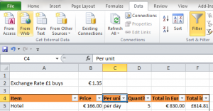
I can filter the items by the ones that match my search criteria, by using the the Filter option in the Data tab.

To filter my budget, I put my cursor on the heading for per unit, and then click on the Filter icon. I know the filter has been applied as down arrows appear next to the heading titles.

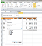
I select the down arrow next to the per unit heading

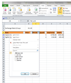
I select the per person filter, by removing the tick from select all and then tick per person, and click OK. Here are my results.

When I want to see all my items listed again, I click on the down arrow next to heading and select Clear filter from per unit.

Remember: It is possible to forget you have the filter on, and then have a minor moment of panic when you think you’ve lost data…I think Excel knows this can happen….so look out for the down arrow next to your heading as a reminder. Excel is thoughtful like that!
Using filters is included in our Excel Intermediate courses under List Management. For more information on our Excel training courses and the course syllabus, please see https://www.stl-training.co.uk/excel-2010-intermediate.php