Microsoft Excel – STL

If you have an Excel Worksheet that contains Data relating to the hours of training for each Employee for Microsoft Excel Training London on Monday, Tuesday and Wednesday, you may want to return the hours trained for a particular employee on a particular day in another Excel Workbook or Excel Worksheet.

The spreadsheet shown below is the data set we will use:

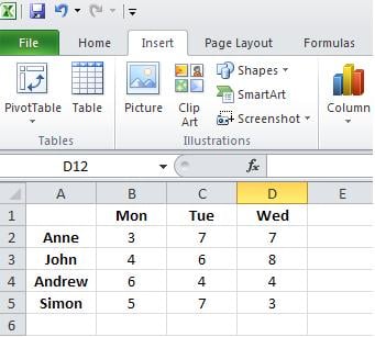
The Excel INDEX function can return an item from a specific position in a table of Excel data using Row and Column headings. The MATCH Function can return the position of a value in a list. The INDEX and MATCH functions used together provide a flexible and powerful method for extracting data from a table.

We start with the INDEX function. The Index function has three arguments(Array,Row_Num,[Col_Num])

The Array argument is the range of cells we are trying to retrieve the data from. The Row_Num argument is the Row you are retrieving from and Col_Num the column you are retrieving from. The value at the intersection point of the Row and Column arguments will be returned from the cell range from the Array argument. We use the MATCH function to assign the Row and Column to the second and third arguments of the INDEX function.

The Match function has three arguments:

(Lookup_Value,Lookup_Array,[Match_Type])

Here is the spreadsheet we will use to create the formula which will return the number of hours. The formula is entered into cell B5 of the Index and Match formula sheet:

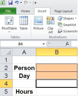
The screenshot below shows the result and notes:

=INDEX(‘[Data Table Excel Workbook.xlsx]Sheet1′!$B$2:$D$5,MATCH(B2,'[Data Table Excel Workbook.xlsx]Sheet1′!$A$2:$A$5,FALSE),MATCH(B3,'[Data Table Excel Workbook.xlsx]Sheet1’!$B$1:$D$1,FALSE))

Enter a value into B2 and a value into B3 of the Index and Match formula sheet and in cell B5 of the Index and Match formula sheet it will return the hours of Excel Training completed for that Employee.

Formula Explanation Notes:

1. The first argument of the Index function relates to just the hourly figures in the Data Table Excel workbook(B2:D5).

2. The Row Argument of the Index function uses the Match function to match the value of cell B2 in the Index and Match Formula sheet to the corresponding value in the Data Table Excel Workbook(A2:A5).

3. The Column Argument of the Index function uses the Match function to match the value of cell B3 in the Index and Match Formula sheet to the corresponding value in the Data Table Excel Workbook(B1:D1).

4.The formula returns the value form the Array argument that represents the row and column values specified.

5. The FALSE statement returns the exact value found.

In the following example there is a column of stock codes. The numbers represent our Supplier and the letters after the hyphen (-) indicates our Item number.

Suppose we need to extract the Supplier and Item codes and place in separate cells. If our Supplier codes were all equal length e.g. 3 numbers long, we could simply use the LEFT function.
In the Excel 2010 Training Courses here in London this is a common question.

Example:

Result:

The problem we have is that not all Supplier codes are 3 numbers in length.
We can correct this by using another Excel function word, FIND.

FIND function can return a number value of where a particular character appears, e.g. if we have a word “BEST-STL TRAINING” the FIND function would tell us that the hyphen is the 5^th character.

We could use this inside (nested) the LEFT function – But remember we do not want to include the hyphen (-) in our final result so we need to subtract 1.

Example:

NOTE: Without subtracting 1 in the above example, it would return a value of 4

Final Code: =LEFT(A2,FIND(“-“,A2)-1)

We could repeat this for the Item code by using a combination of RIGHT, LEN and FIND nested.

Blog Categories