Categories
Excel Training

Excel Training: Use Goal Seek for What If Scenarios

Excel has some great functions for “What if…” scenarios. One tool that can be used is the Excel Goal Seek. This allows you to choose any current formula and set the answer value to your own goal.

e.g. If you have a formula that works out how much profit you make from selling items, such as £20, but you would like it to be £30 profit, Goal Seek can change various cells to achieve that £30 goal.

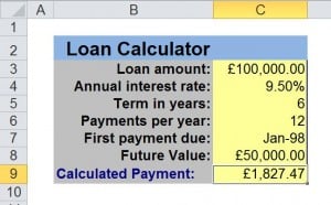
Below is an example similar to ones we use on our Excel Training courses based in London. We have a simple loan calculator that uses the PMT function to work out monthly loan repayments.

Excel Goal Seek Tool


Open the Goal Seek from the Data Ribbon, Data Tools Section, What If Analysis.

Excel Data Tools Goal Seek Ribbon Bar

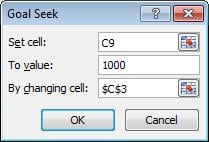
The Goal Seek dialog appears. Fill out as follows: Enter the cell you wish to set your goal to in Set Cell Field. Enter the figure you want the Goal to achieve in the To Value Field. Enter the variable (cell) you would like Excel to change to reach your set Goal in the By Changing Cell Field.

Excel Goal Seek ToolClick OK

The Sheet content will change to reflect the Goals set. You will be presented with another dialog box, Click OK to keep the changes, or Click Cancel to revert the cells back to original values.
 

Categories
Excel Training

Using COUNTIFS with Excel 2003

Excel 2007 introduced the function COUNTIFS to count cells based on multiple criteria.

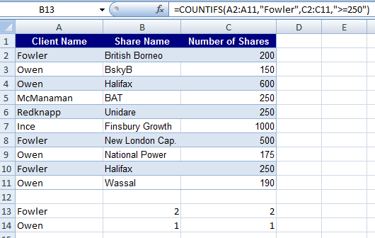
For example suppose you wish to count how many times the client Fowler buys more than 250 shares. The answer for tha data below turns out to be 2 using the Countifs function entered in B13.

Similarly for Owen the result turns out to be 1. 


Even though COUNTIFS is not availailable with Excel 2003 there is an alternative way to perform the same calculation using the SUMPRODUCT array formula.

The formula

 =SUMPRODUCT(–(A2:A11=”Fowler”),–(C2:C11>=250))

typed into C13 produces the same result. The mysterious looking — operator calculates if true or false for each of the cells in the range A2:A11 returning 1 if true and 0 if false. The same goes for the range C2:C11 and the Sumproduct array function sums all the true, true (1*1) combinations.

Note – To show how — works try typing –(A2:A11=”Fowler”) into a cell followed by Ctrl+Shift+Enter. This convets the formula into the array formula {=(A2:A11=”Fowler”)}