One of the great new features of Excel that users enjoy employing during our Microsoft Excel Courses here in London is the Sparklines. These can be thought of as mini-Charts that reside in a cell, and can show a trend visually of a group of values.
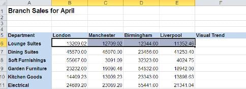
In the example shown below there are sales figures from four store locations, London, Manchester, Birmingham and Liverpool. We want to see the trend of these figures visually beside each Department row, rather than create a separate Chart.
Start by selecting the range of cells required for the Sparklines. In the example above, Cells B6:E6.
From the Insert Ribbon select the Sparkline style required e.g. Line
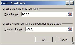
The Create Sparklines dialog appears.
Select the location where the Sparkline should be displayed e.g. F6
Click OK – The Sparkline will appear in the chosen cell as seen below.
With the Sparkline cell selected you will see the Sparkline Ribbon – Design.
From this Ribbon you can chage the appearance and type of Sparkline e.g. from Line to Column or Win/loss.
Once the format has been completed you can copy the Sparkline to reflect other values, by copy/paste or using the AutoFill.
Sparklines are not visible in earlier versions of Excel (prior to 2010).
The Sparklines option will not be available if a Workbook is opened in Compatibility Mode.


