An easy to update Gantt chart in Excel
Building a Gantt chart in Excel is pretty easy. But what if you needed to update any of the tasks? This would usually mean lot’s of time consuming manual editing of cells. But there is an easier way….
Step in Excel and the ever flexible conditional formatting function! Yes by deploying some neat conditional formatting tricks you can produce a presentable usable Gantt chart in Excel. You can also learn conditional formatting by attending Microsoft Excel training course.
Recap: A Gantt chart is made up of task bars, one for each of the tasks required to complete the project in hand. The task bars typically have start and finish dates and therefore have different lengths on duration.
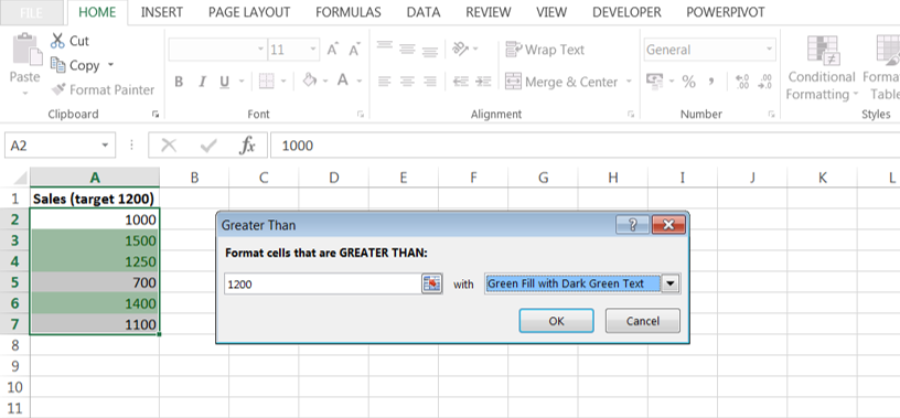
By using Excel’s Conditional Formatting feature we can create our project task bars for our Gantt chart. We will be able to different colour task bars conveniently managed by conditional formatting. An example is shown below on how cell colours can be changed; sales figures green if they exceed a target figure of 1200.
Let’s create a Gantt chart in Excel
By using conditional formatting we can easily create the following.
Creating the conditional formatting rule
Step 1. Start by selecting the range of cells where bars are to be displayed. In the above example range F2:T11.
Step 2. Select the Home tab then choose Conditional Formatting.
Step 3. Pick New Rule then Choose a formula to determine which cells to format.
In the empty box box (format values if formula is true) enter the formula:
=AND($D2<=F$1,$E2>=F$1)
This formula returns True if a task Start Date is before or equal to the chart date (entered in row 1) AND the Finish Date is after or equal to the chart date.
AND means both conditions within the brackets must apply. The $ sign before a letter means keep that column fixed when applying the rule to the range of cells. Similarly, the $ before a number means fix that row when applying the rule.
Step 4. Now click the Format button and choose a fill colour then OK.
In the example all cells that obey the rule are coloured blue.
Adding more rules
Additional rules can be added for example if certain tasks are designated critical by typing CT in the C column then colour the bars pink.
To do this create a new rule as before but include a third condition where the type is CT.
=AND($D2<=F$1,$E2>=F$1,$C2=”CT”)
Click Format and choose pink as the fill colour.
Tips
For consistency you can choose specific fill colour by selecting Fill, More Colours, Custom then entering 255,153,255 for Red, Green and Blue.
Adding a white top and bottom border as part of the Formatting rule can help to separate the bars when touching.
To make changes to colours or to formulas you must highlight the exact range containing the conditional formatting then select Conditional Formatting, Manage Rules. To help do this quickly select Home, Find & Select, Conditional Formatting.
Conditional formats can be copied using the Format Painter.
Additional Resources
Present your data in a Gantt chart in Excel
Pro tip: Create a Gantt chart in Excel


