excel – Page 19 – STL

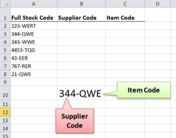
In the following example there is a column of stock codes. The numbers represent our Supplier and the letters after the hyphen (-) indicates our Item number.

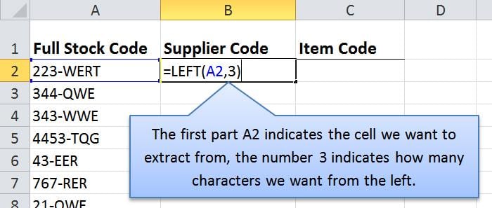
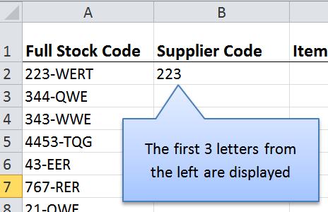
Suppose we need to extract the Supplier and Item codes and place in separate cells. If our Supplier codes were all equal length e.g. 3 numbers long, we could simply use the LEFT function.
In the Excel 2010 Training Courses here in London this is a common question.

Example:

Result:

The problem we have is that not all Supplier codes are 3 numbers in length.
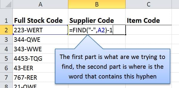
We can correct this by using another Excel function word, FIND.

FIND function can return a number value of where a particular character appears, e.g. if we have a word “BEST-STL TRAINING” the FIND function would tell us that the hyphen is the 5^th character.

We could use this inside (nested) the LEFT function – But remember we do not want to include the hyphen (-) in our final result so we need to subtract 1.

Example:

NOTE: Without subtracting 1 in the above example, it would return a value of 4

Final Code: =LEFT(A2,FIND(“-“,A2)-1)

We could repeat this for the Item code by using a combination of RIGHT, LEN and FIND nested.

Ever closed an Excel workbook and clicked the “Don’t Save” option, then realised you should have saved it! Microsoft Excel 2010 now has a file recovery option for just such an occassion. This has proved invaluable in our Microsoft Excel Training Courses in London.

Always check the AutoRecover time in the Excel options. To do this go to the File, Options and Save. (Shown below)

Set the “Save AutoRecover information every” time to 2mins.

Retrieving a workbook after it’s been closed without saving can be achieved by:

File Ribbon, Info

From the Info panel select the Manage Versions button, then Recover UnSaved

A list of unsaved documents will be seen. Select the one required.

Note: This works for both documents that you have previously saved, and docs never saved

Blog Categories