Categories
Excel Training

Excel Training: Sum Visible Cells Only in Excel 2007 and 2010

A question that often arises when using AutoFilter with Excel is… how can I sum the visible data only? The solution to this question may not always be apparent but all is not lost as there are many Excel training courses in London that deal with how this can be achieved.

There are 2 options for you to do this.

Option 1

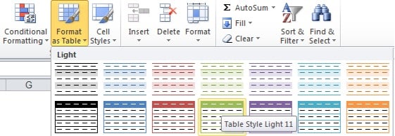
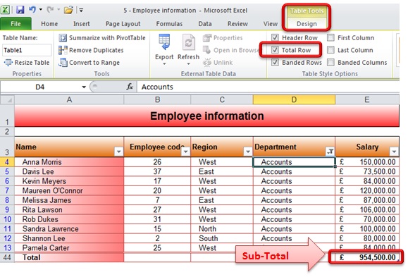
Format the data as a table. To do this go to the Home ribbon and from the Styles group click on ‘Format as Table’. Select the table style you require, then, add the total row from the ‘Table Style Options’ group in the Options ribbon. Now, whenever you filter the data the resulting totals will only be shown for the visible cells.

Excel Training Format Data as a Table

Excel Training London Sub-Totals for Tables


Option 2

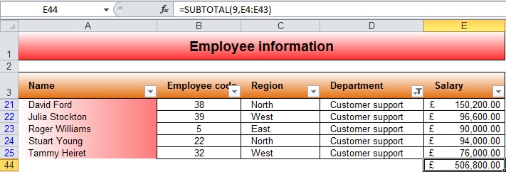
2) Should you not wish to work with the data formatted as a table then, apply a filter first, add the totals you require in the row of blank cells below the visible cells. Use the AutoSum  tool for this purpose which will create SUBTOTAL functions calculating the visible cells only. When you clear the filter the totals now shown will be for all the data. Adding a new filter will show the totals for the data that is visible.

The 2nd option can also be used in Excel versions before 2007.

Excel Training London Data Sub-Totals


Since there are so many different things that one can do in Excel, it is extremely important to take advantage of the Excel training courses available in London which cover the most useful tools and functions.
Categories
Excel Training

Excel Training: Use Goal Seek for What If Scenarios

Excel has some great functions for “What if…” scenarios. One tool that can be used is the Excel Goal Seek. This allows you to choose any current formula and set the answer value to your own goal.

e.g. If you have a formula that works out how much profit you make from selling items, such as £20, but you would like it to be £30 profit, Goal Seek can change various cells to achieve that £30 goal.

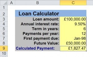
Below is an example similar to ones we use on our Excel Training courses based in London. We have a simple loan calculator that uses the PMT function to work out monthly loan repayments.

Excel Goal Seek Tool


Open the Goal Seek from the Data Ribbon, Data Tools Section, What If Analysis.

Excel Data Tools Goal Seek Ribbon Bar

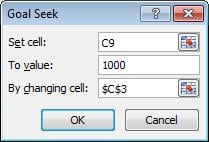
The Goal Seek dialog appears. Fill out as follows: Enter the cell you wish to set your goal to in Set Cell Field. Enter the figure you want the Goal to achieve in the To Value Field. Enter the variable (cell) you would like Excel to change to reach your set Goal in the By Changing Cell Field.

Excel Goal Seek ToolClick OK

The Sheet content will change to reflect the Goals set. You will be presented with another dialog box, Click OK to keep the changes, or Click Cancel to revert the cells back to original values.