On a recent Excel VBA Intermediate course everyone thought a macro for converting text to upper or proper case would be helpful. It’s a good one to put into your Personal Macro Workbook then assign to a button on your Quick Access Toolbar. Here’s how to do it:
1. Starting with a blank Workbook record a macro called ConvertCase in the Personal Macro Workbook. With Excel 2007 or Excel 2010 click View, Macros, Record Macro…
2. Press OK then straight away click Macros, Stop Recording.
3. Press Alt+F11 to view the VBA Editor and open the module and code window for the blank ConvertCase macro.
4. Now add the following code:
Sub ConvertCase()
‘Macro to start frmConvertCase
frmConvertCase.Show
End Sub
Sub Uppercase()
For Each rng In Selection
rng.Value = UCase(rng.Value)
Next rng
End Sub
Sub Propercase()
For Each rng In Selection
rng.Value = Application.WorksheetFunction.Proper(rng.Value)
Next rng
End Sub
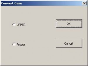
5. Insert a User Form and name it frmConvertCase using the Properties window adding a caption ‘Convert Case’.
6. Add two Option buttons and two Command buttons to your form:
7. Name the controls Upper, Proper, OK and Cancel adding captions as shown below.
8. Double click the OK button and add the following code:
Private Sub OK_Click()
Dim rng As Range
If UPPER.Value = True Then
Call uppercase
ElseIf Proper.Value = True Then
Call propercase
Else
MsgBox “Please choose either upper or proper case”
End If
End Sub
9. Close the code window the double click the Cancel button adding the following code:
Private Sub Cancel_Click()
Unload frmConvertCase
End Sub
10. Finally close the VBA Editor and customise your Quick Access Toolbar.
Select More Commands, Choose commands from Macros and select your ConvertCase macro, Add, OK.
That’s it. You now have a permenant button to change case of any selected text!
