Excel Functions Resources

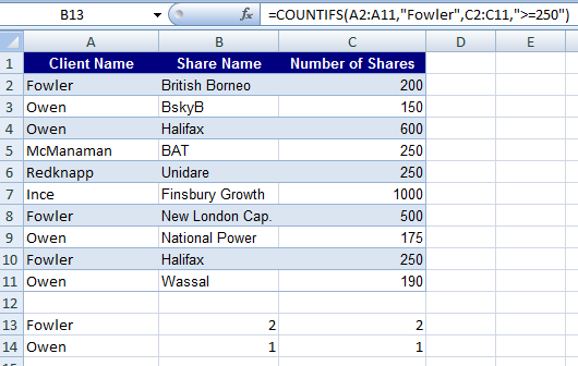
It’s easy to fall into a habit, and manually type in a formula and copy and paste it within a worksheet. If so, you may not be getting the most out of the Formula tab on the Ribbon. From here, you can save yourself time by using Excel’s ready made formulas using Functions. The Formulas tab has […]

Excel 2007 introduced the function COUNTIFS to count cells based on multiple criteria. For example suppose you wish to count how many times the client Fowler buys more than 250 shares. The answer for tha data below turns out to be 2 using the Countifs function entered in B13. Similarly for Owen the result turns out to be 1.            […]