Categories
Excel Training

Excel Charts – beginner’s guide to creating a pie chart

I’m new to the charting side of things…I’m used to staring at numbers on worksheets and trying to figure out what it all means…and admiring those around me who use charts…so mysterious…so professional looking…so much nicer than my rows of figures.

Charts make it so much easier to spot trends and analyse data – and I felt that the time had come to take a bite of that pie.  The idea of adding a chart filled me with a sense of dread…so I decided to  experiment with some basic charting to prove that it was possible to do, and all without the aid of several cups of coffee and a pep talk.

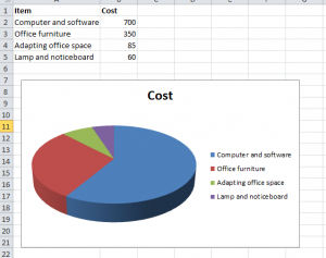
So here’s what I did.  As a simple example, I decided to look at how a pie chart could represent the cost of items in a range of categories for a (fictional) home office.
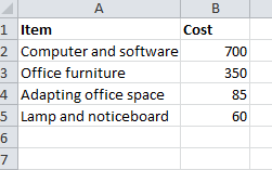
data-to-make-simple-chart-for-excel
Basic data for creating a small home office

I can show this data in a more visual way using a chart.  I can access charting options via the Insert ribbon. The first step is to decide on  the kind of chart I want, so I’m opting for a pie chart to make it easier to compare the proportional costs involved.

So, I select the data above and then go to the Insert ribbon, and click on the Pie Chart icon.   Because I’m feeling particularly brave, I’ve opted for the 3D pie chart…and it looks like this….
example-of-3d-piechart-cost-comparison-excel-training-intro-level
Here is my first attempt at using a 3D pie chart to show the costs involved in creating a home office.

It is a basic example, but it proved to me how easy it was to insert a chart – it took less than a minute to do.  Now…what can I chart next…


Categories
Excel Training

Adding a Calculated Item to a Pivot Table in Excel 2010

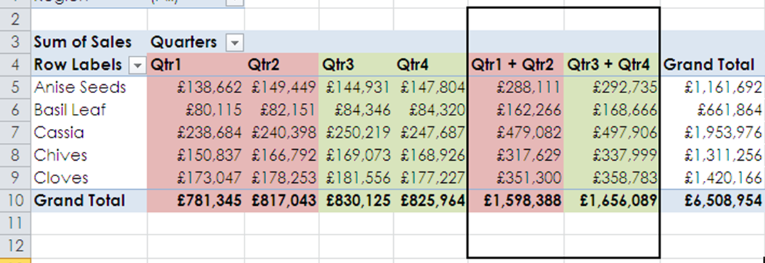
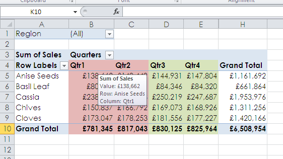
Above is an example of a standard pivot table in Microsoft Excel 2010.  It is set up with financial quaters as column headers and products as Row labels.  I’m interested in seeing the results for the combined sales for the first half and the second half of the year. As you can see I have colour coded these two halves and now I am going to add two “calculated items” showing a total for Q1+Q2 and Q3+Q4.

TAKE ACTION: 

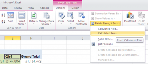
  1. Ensure your cursor is placed onto the Q4 column header as in the image.
  2. Select the “PivotTable tools” tab and click on “options”
  3. In the “calculations” box” select “fields, items, & sets” and then “calculated items”

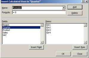
When this box appears follow these instructions:

  1. Click into the “name” field and enter the new name Qtr1+Qtr2.
  2. Click into “formula” field, remove the 0, double click on Qtr1 in the “Items” field, add + then double click on the Qtr2 from the “Items” field.  Here you are entering a formula which is Qtr1 + Qtr2.
  3. Click the “Add” button and then OK

You will now see that this new column has been added to your PivotTable in Microsoft Excel 2010.

Repeat this process for Qtr3 + Qtr4 and adjust the background colours to match those already on the pivot table.  All going well you should have a pivot table that resembles the one I have pasted below:

You now have a pivot chart showing you the totals for both halves of the year.  Take note that your grand total includes your two new columns so its best to remove that. To learn how to remove the total column in Microsoft Excel 2010, well that’s for the next blog.

Good luck!