Most Excel users do not know the power of custom formatting. They know how the currency or accounting format. In this article you will find some useful information which can display your data in different ways, and more clearly.
I got the inspiration to write this blog post from a client question on one of my Excel courses.
The client asked me “I get data from our financial system. In one column I have a percentage, but the column is not percentage formatted. When in Excel, I add percentage formatting, Excel multiply the numbers by 100. I don’t want to have to divide the column by 100. Do you have a solution?”
IMPORTANT: CUSTOM FORMATTING WILL NOT CHANGE THE DATA ONLY CHAGE HOW EXCEL WILL DISPLAY THE DATA.
To create custom formatting in Excel:
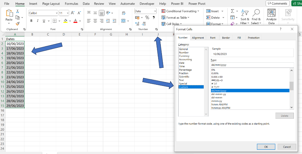
Select the data and click the down arrow bottom right corner of the Number group on the ‘Home’ ribbon. In the Format Cells dialog box click Custom bottom left.
In this example you will see an example of dates custom formatting.
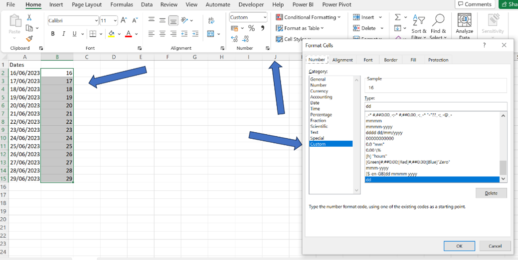
You will have to type the code. When it comes to custom formatting for dates dd display day number.
If we enter “dd” in the Type box Excel will only display the day number.
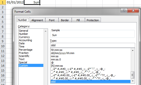
Alternatively, if we type “ddd” in the Type box, Excel will display the first 3 letters of the day name.
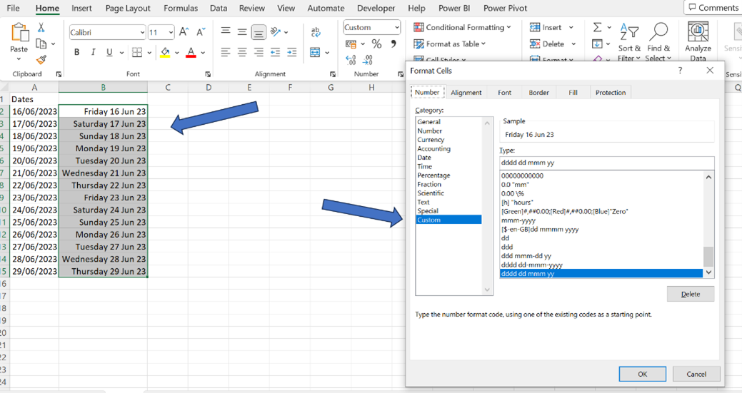
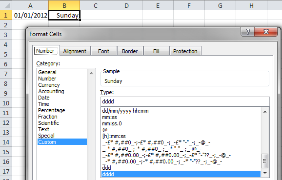
4 times d will display the full day name. Use ds for days, ms for moths, and ys for years.
The code dddd dd mmm yy will then display:
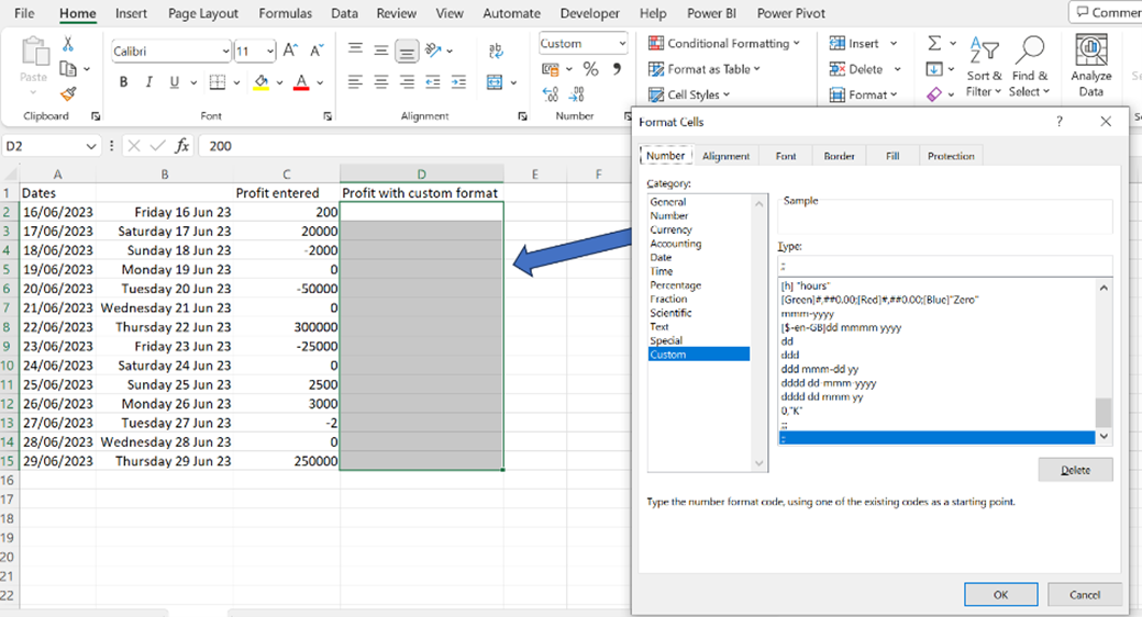
In the next example you will see some options for numbers.
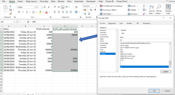
;; will display the cells like they are empty.
If you only want to display positive numbers use the code 0;;
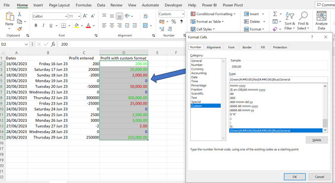
What you have in front of the first semicolon (;) define positive numbers, between the two semicolons define negative numbers, and after the second semicolon define zero. A colour inside square brackets can define font colours. The code [green]#,##0.00;[red]#,##0.00;[blue]0 will result in positive numbers being in green. # are optional digits. So, with a number above 999 you will get thousands separator. You will always get two decimals. Negative numbers will be in red and zeros blue.
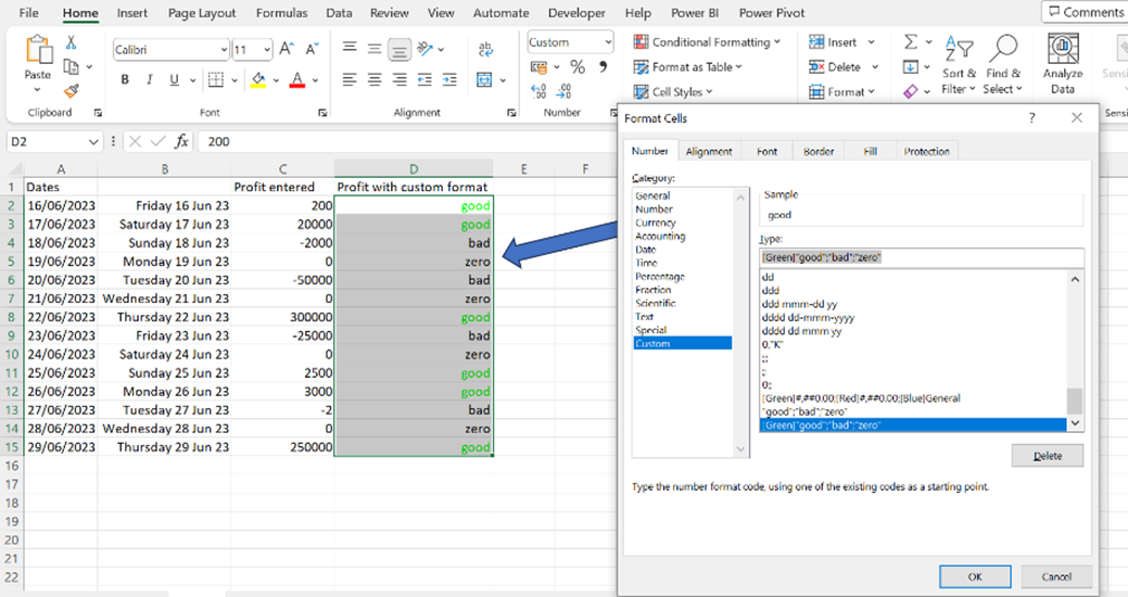
When you have zero in the code, you tell Excel that you want to display the number, but you can also turn it into text only. The code [Green]”good”;”bad”;”zero” will not display any numbers.
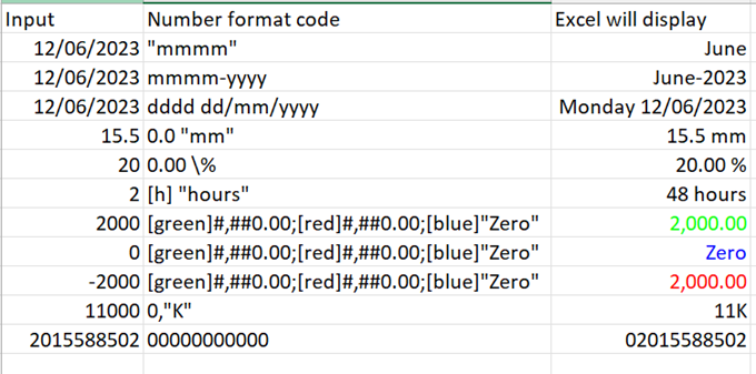
You can find a table of examples below, but it is endless what you can get Excel to display.
Conclusion
Custom formatting in Excel is useful for numerous reasons. Primarily, it can help improve the visual appearance of your data and make it more readable.
Custom formatting can help save time and reduce errors by automatically applying specific formatting to your data. For example, you can use custom formatting to automatically add a “%” symbol to values entered in a certain column.
Custom formatting can help you better communicate information in your data by allowing you to display it in a more meaningful way. For example, you can use custom formatting to display dates in a specific format or to display times with AM or PM.
Overall, using custom formatting can make your Excel data look more professional, easier to read, and more informative.

