Slicers you will be able to depict the datasheet fields more comprehensively. Excel 2010 include this feature for the first time, which lets you to slice your data by showing you only the element stored in the tables. Real usage of Slicers can be seen with pivot table. Unlike Pivot table, which pivots down the datasheet, it makes you to compare and evaluate the data from different perspectives. This post will explain how you can use Slicer with Pivot Table and Charts.
To begin with, launch Excel 2010, and open a datasheet, containing Pivot Table.
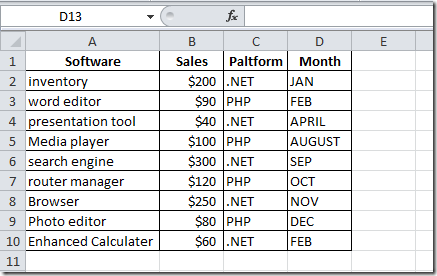
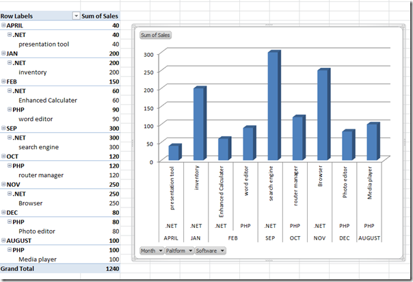
We have made Pivot Table and Pivot Chart using the above datasheet.
The datasheet, containing fields; Software, Sales, Platform, and Month. Datasheet shows the software developed using two platforms (PHP, .NET), its price and month in which development completed.
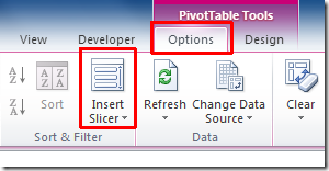
Now we want to create slicers for each category present in Pivot table. For this, select the whole Pivot table, and navigate to Options tab, click Insert Slicer.
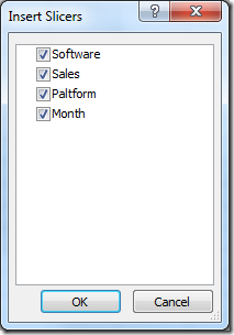
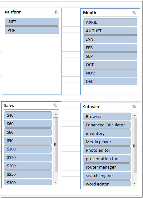
Upon click, Insert Slicers dialog will appear, containing fields of the Pivot table. Select the desired one from the list to view respective Pivot table and chart, and click OK.
You will see box of each field, containing data as shown in the screen shot below.
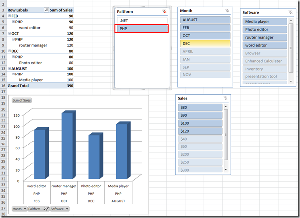
Now we want to view the software developed on PHP platform. For this, we will click PHP in Platform field box. You will see the pivot table and chart will automatically show all the info related to PHP platform, i.e, in which month it was used, which software developed on this platform and price of the software.
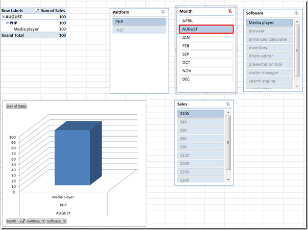
Now if we select August from Month field, then it will show all the info related with month of August, i.e, which platform was used to make which software, and what was its price.
By using Slicers you can filter down your data in more detail. Its real usage can be seen when you are dealing with huge data sheet.
Want to become an Excel expert? Attend one of Best STL’s Excel 2010 training course available London and UK wide.
