Charts from a dropdown list

Charts from a dropdown list in Excel

Many people who use Excel can generate a chart or two on their spreadsheets. This is a relatively easy task to perform in Excel. These charts will either sit in data sheets or in their own sheets.

Don’t you sometimes wish you had a button to click in Excel which gives you a list of charts to display on your sheet? Well, I can show you how to do this!

Just to let you know, you can do an excel course with us to learn this in practice.

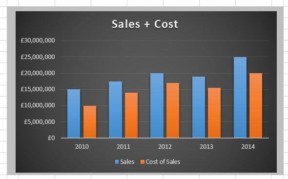
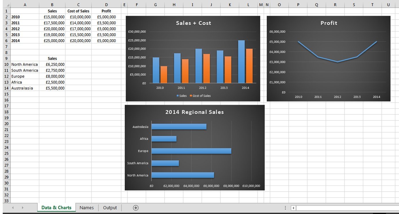
First of all, you will need some charts. It doesn’t matter which types of charts they are. The screenshot below shows an example of a sheet containing data and charts:

Once you have your charts up and running, you can begin to build your interactive button. The first thing you need to do is to select the cells which are behind the first chart, as shown below.

After doing this, click in the Name box (top left next to the Formula bar). In here, give this selection of cells a name, for instance Sales. Do the same for all the other charts you wish to add to the list. These names will be used later to choose the right chart from the list. Now, in a different place on the sheet, or in another sheet, type a list of your chart names you want to display in the dropdown box (see my example below ).

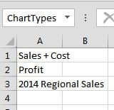
Select this list and give it a name (in the Name box again), as shown above. This name will be used to generate the dropdown list. We are now ready to create the dropdown button. Add a new sheet to the workbook and name it Output. Activate the Developer tab in the ribbon. Click File – Options – Customize Ribbon, then tick the box next to Developer in the right hand side box. Select the Developer tab in the ribbon, then click the Insert button.

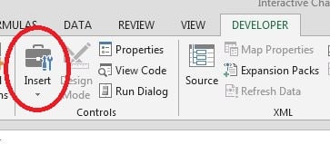
This opens a toolbox from which you select the Combo Box item. Now, in the Output sheet, draw the Combo Box near the top of your sheet with your mouse. Afterwards, press Ctrl+1 (format control). A dialogue box opens as shown below:

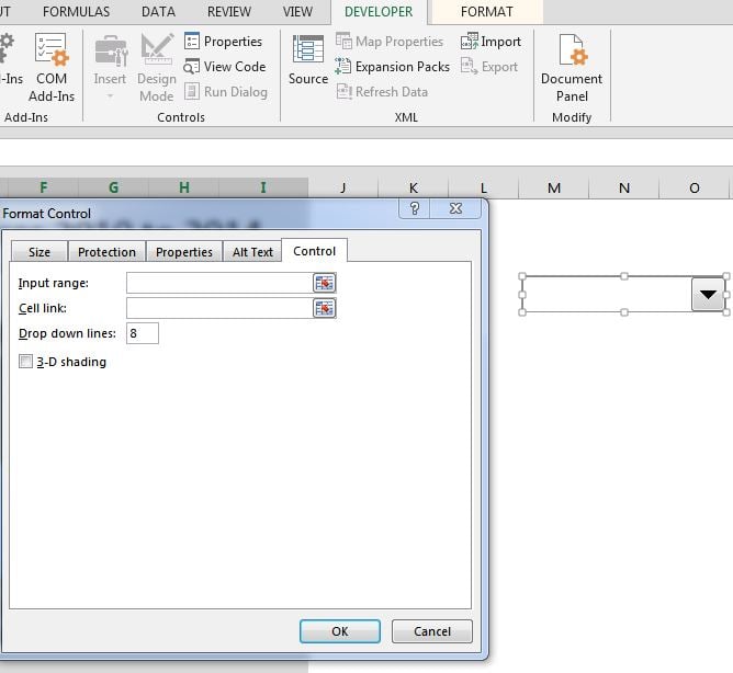
Click in the Input range box and then type the name which you gave earlier to your list of charts  (I called mine ChartTypes). Next, click in the Cell link box, then click in any empty cell in your spreadsheet. This cell reference now sits in the Cell link box. We shall use this cell later to pick a chart.

The next thing we need to do is to define a name which uses Excel’s Choose function to pick the correct chart from the list.

Step 1: Select the Formulas tab, then select Define Name.

Step 2: Type SelChart into the Name box. (SelChart is my example)

Step 3: Type the following into the Refers To box:    =choose(                                                            Now select the cell you selected for the Cell link box earlier. Next, type the names you gave your charts in the Name box.

=choose(selected_cell,Name1,Name2,Name3)  (selected_cell is the cell you used in the Cell link box earlier. The other names are the names you gave the cell ranges behind your charts.)

Step 4: Click OK.

Almost there! We now need to again select the cells behind each chart, (one chart at a time), then right-click the selection. In the dialogue box, click Copy, then go to your Output sheet. Right-click below your dropdown combo box and select Paste Special – Linked Picture. (See below)

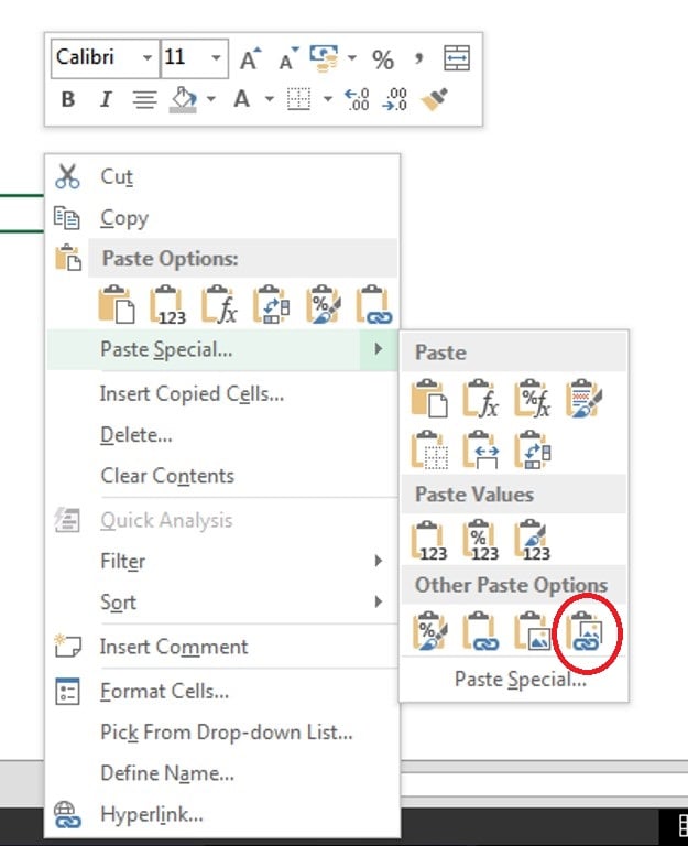
Hopefully, you now have an image of your chart in that location on your sheet. Click in the formula bar and type =SelChart (again, this is my example). Press Enter. Do this for all your charts. Now you can create Charts from a dropdown list.