Categories
Excel Training

Using number filters in Excel

I can filter data in my Excel worksheet, using the number filters.  This is another time-saving feature that helps me to get the data I need, quickly and easily.

list-of-students-course-on-excel-2010-training-course
The list of students

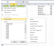
You can access the number filters, by selecting the down arrow next to the filter in the column you want to review.
number-filters-in-excel-2010-training-courses
Number filter options – so you can get the information you need in one click.

The filters offer you the apply number filters including:

  • Equals
  • Does not equal
  • Greater than
  • Greater than Or Equal to
  • Less than
  • Less than or equal to
  • Between
  • Top 10
  • Above average
  • Below average

If you click on a number filter, a dialogue box will open and you can type in the figures to complete your task.

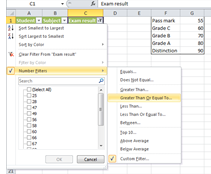
For example, I want to sort my list by those students with results between 55 and 70.
number-filter-greater-than-or-equal-to-excel-2010-training-courses
Filter options appear when you click, to figure out results between 55 and 70. I’m going to use “Greater than Or Equal to”

Excel now gives me a dialogue box and I can add the range I want to find, and use the additional options in this box to customise my search.

add-values-to-filter-excel-2010-training-courses
Setting up the range using number filters

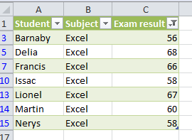
Once I press ok, Excel gives me the results.
results-from-filter-excel-2010-training-course
The results using the filter.

Using filters is included in our Excel 2010 training courses.  Take a look at what you can learn https://www.stl-training.co.uk/syl/26/excel-formulas-functions.html


Categories
Excel Training

Use conditional formatting to analyse data in Excel

An experiment using conditional formatting…

I have a list of fictitious students who have taken an Excel exam this morning. The pass mark was 55, but I want to help the whole group to achieve a Grade B with a pass mark of over 70%.

I want to be able to find who needs to attend an extra workshop to help boost their skills and get them to 70%.  I can identify the students quickly by using conditional formatting.

Here is my list of students and their grades

list-of-students-course-on-excel
List of students and their exam results.

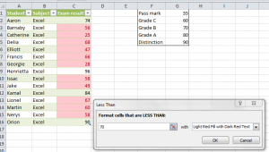
I want to find all those students whose grades were under 70.  I select my table, and then, use the Home tab, Conditional Formatting, and select Highlight Cells Rules, then select Less than.  A dialogue box appears and I need to put in the value.  I type in 70, as I want to know all the scores below 70, and press ok.

Highlight-results-below-70-course-on-excel
The dialogue box appears and I can type in the score. Excel will then identify all the results less than that value.

I now know, that out of 15 students, 13 would find a workshop helpful to boost their skills.  I can now set up the room, and the trainer can target his course on Excel to help the students reach their target score.

I can use the filter in my table to give the trainer the names of the students for his session.

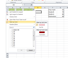
I go to the filter arrow on the results column and select filter by colour

filter-by-colour-course-on-excel
Filter by colour – is a quick way for me to create a delegate list for the session.

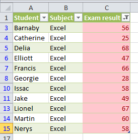
Here is my workshop attendance list, with the 13 students names.

Final-list-filter-by-colour-course-on-excel
Here is my final list.

This is a quick way to experiment with analysing data using conditional formatting, and using the filter to pick out the data you want (and hide the data you don’t need at that moment).  A course on Excel is a convenient way to upgrade your skills and experiment with data before you try it out in the workplace.  https://www.stl-training.co.uk/microsoft/excel-training-london.php