Categories
Excel Training

What are contextual tabs in Excel?

I was on an Excel Intermediate course last week, and I noticed that when I was working with a chart, specific tools appeared.  When I clicked out of my chart, the tools would disappear…What is going on Excel?  Why are you doing that?  How do I get them back?  (Mild panic followed…”have I broken it?”)

Fortunately, my calm and understanding trainer explained that these disappearing tools are called contextual tabs.  And no, Excel doesn’t hide them to induce Excel-panic, it is actually being pretty smart.

Contextual tabs appear when you are creating or editing an object like a chart, or table or even a diagram in Excel.  The contextual tabs give you the options and tools you need to work with these objects and then when you click out of the object the tools are tidied away.  To get them back, you click on the object, and the tab appears again.  It keeps your working space uncluttered.
contextual-tab-visual-basic-excel-training
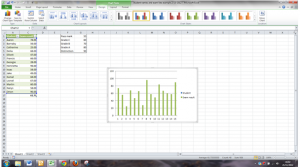
The green tab is a contextual tab, that appears when I’m working with my chart.

In the above screenshot, I’ve put a chart into my document, and you can see a green highlighted tab – this is the contextual tab which I can use to amend my chart.  When I click out of my chart, and back into my spreadsheet, the contextual tab disappears.
no-contextual-tab-visual-basic-excel-training
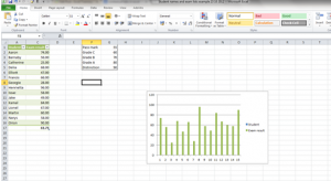
When I click out of my chart, the contextual tab disappears…look! the green highlighted tab isn’t there…

See if you can spot the difference!

Getting used to what Excel does, and when, is really essential – I can get more out of it if I understand why it does these strange things. Contextual tabs stop winding me up when I know why they appear, and why they don’t.

When I’m ready, after a bit more practice, I’m going to try visual basic Excel training – but for the next few weeks, I’m going to keep experimenting with what I’ve learned so far.  If you want to lose the Excel-panic or just get more out of the program, take a look at what the courses cover on https://www.stl-training.co.uk/excel-vba-2010-training-course.php.
Categories
Excel Training

How to correct names in lower case in Excel (Proper Case)

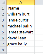
It can be a pain when you have a list of names that are all in lower case, and you want to be able to change them to the right case.  This can be easily completed using a formula to make the changes.

names-lowercase-excel-vba-courses-london

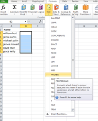
To change this list of names to the proper case, I can use one of Excel’s off-the-peg Text formulas by using PROPER.

proper-formula-excel-vba-courses-london
The Proper formula in the Formulas tab.

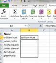
To apply this, I need to use an empty column (in this case B) to apply the formula to the original names.  This is only temporary as I will copy the names back into Column A when it’s all done.

I click on cell B2 to set up my formula.  I go to the Formulas tab, and select Text Formulas, and PROPER.

A dialogue box appears, and I can now select the first name in column A.

active-cell-excel-vba-courses-london
selecting the cell contents that need to be changed

When I click ok, the first name is now in the correct case.  I can copy this formula by using the autofill handle, to complete the changes to the remaining names.

Autofill-formula-excel-vba-courses-london
Autofilling the formula to the remaining cells

The names have all be corrected and I can copy them from column B back into column A.

Our Excel courses cover all levels from introduction to advanced, including Excel VBA courses london, https://www.stl-training.co.uk/vba-training-london.php.