Categories
Excel Training

Adding a Calculated Item to a Pivot Table in Excel 2010

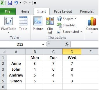
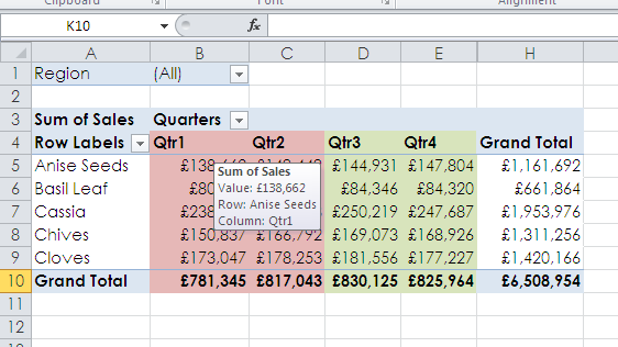
Above is an example of a standard pivot table in Microsoft Excel 2010.  It is set up with financial quaters as column headers and products as Row labels.  I’m interested in seeing the results for the combined sales for the first half and the second half of the year. As you can see I have colour coded these two halves and now I am going to add two “calculated items” showing a total for Q1+Q2 and Q3+Q4.

TAKE ACTION: 

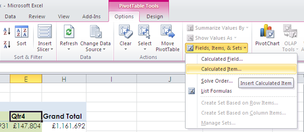
  1. Ensure your cursor is placed onto the Q4 column header as in the image.
  2. Select the “PivotTable tools” tab and click on “options”
  3. In the “calculations” box” select “fields, items, & sets” and then “calculated items”

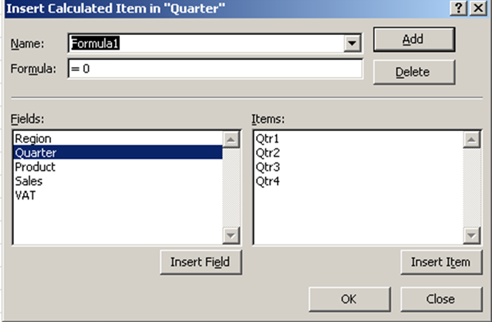
When this box appears follow these instructions:

  1. Click into the “name” field and enter the new name Qtr1+Qtr2.
  2. Click into “formula” field, remove the 0, double click on Qtr1 in the “Items” field, add + then double click on the Qtr2 from the “Items” field.  Here you are entering a formula which is Qtr1 + Qtr2.
  3. Click the “Add” button and then OK

You will now see that this new column has been added to your PivotTable in Microsoft Excel 2010.

Repeat this process for Qtr3 + Qtr4 and adjust the background colours to match those already on the pivot table.  All going well you should have a pivot table that resembles the one I have pasted below:

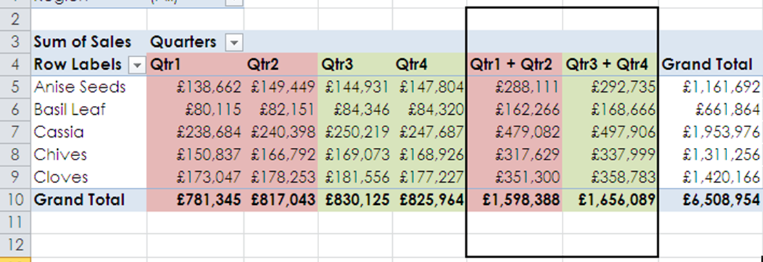
You now have a pivot chart showing you the totals for both halves of the year.  Take note that your grand total includes your two new columns so its best to remove that. To learn how to remove the total column in Microsoft Excel 2010, well that’s for the next blog.

Good luck!


Categories
Excel Training

Excel Courses – Retrieve Data using the Index and Match Functions


If you have an Excel Worksheet that contains Data relating to the hours of training for each Employee for Microsoft Excel Training London on Monday, Tuesday and Wednesday, you may want to return the hours trained for a particular employee on a particular day in another Excel Workbook or Excel Worksheet.

The spreadsheet shown below is the data set we will use:

Data Table Excel Workbook


The Excel INDEX function can return an item from a specific position in a table of Excel data using Row and Column headings. The MATCH Function can return the position of a value in a list. The INDEX and MATCH functions used together provide a flexible and powerful method for extracting data from a table.

We start with the INDEX function. The Index function has three arguments(Array,Row_Num,[Col_Num])

The Array argument is the range of cells we are trying to retrieve the data from. The Row_Num argument is the Row you are retrieving from and Col_Num the column you are retrieving from. The value at the intersection point of the Row and Column arguments will be returned from the cell range from the Array argument. We use the MATCH function to assign the Row and Column to the second and third arguments of the INDEX function.

The Match function has three arguments:

(Lookup_Value,Lookup_Array,[Match_Type])

Here is the spreadsheet we will use to create the formula which will return the number of hours. The formula is entered into cell B5 of the Index and Match formula sheet:

Index and Match formula sheet


The screenshot below shows the result and notes:

=INDEX(‘[Data Table Excel Workbook.xlsx]Sheet1′!$B$2:$D$5,MATCH(B2,'[Data Table Excel Workbook.xlsx]Sheet1′!$A$2:$A$5,FALSE),MATCH(B3,'[Data Table Excel Workbook.xlsx]Sheet1’!$B$1:$D$1,FALSE))

Enter a value into B2 and a value into B3 of the Index and Match formula sheet and in cell B5 of the Index and Match formula sheet it will return the hours of Excel Training completed for that Employee.

Formula Explanation Notes:

1. The first argument of the Index function relates to just the hourly figures in the Data Table Excel workbook(B2:D5).

2. The Row Argument of the Index function uses the Match function to match the value of cell B2 in the Index and Match Formula sheet to the corresponding value in the Data Table Excel Workbook(A2:A5).

3. The Column Argument of the Index function uses the Match function to match the value of cell B3 in the Index and Match Formula sheet to the corresponding value in the Data Table Excel Workbook(B1:D1).

4.The formula returns the value form the Array argument that represents the row and column values specified.

5. The FALSE statement returns the exact value found.