Save hours and eyesore by using freeze panes in Excel
Reviewing data in spreadsheets can be very demanding on the eyes and time consuming when you are trying to remember what a particular column or row of data actually is!
If you’re not already familiar with how to freeze panes in Excel, read on and save yourself some time.
Using freeze panes
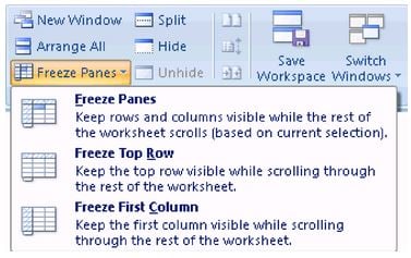
To use Freeze Panes, open a workbook window, and click the Freeze Panes button on the View tab.
Clicking this button will display a menu of freeze options that you can choose from.
To freeze panes (columns and rows)
- Select the first cell of data (for the area you wish to scroll through, not frozen!)
- Go to the View tab
- In the Window group, select Freeze Panes
To freeze panes (top row only)
- Go to the View tab
- In the Window group, select Freeze Top Row
To freeze panes (first column only)
- Go to the View tab
- In the Window group, select Freeze First Column
To unfreeze panes (any setting)
- Go to the View tab
- In the Window group, select Unfreeze Panes
By using freeze panes the time you save over multiple uses really can mean hours saved in the long run. This feature is also particularly useful when sharing Excel spreadsheets with others so as to enable easier navigation and hopefully comprehension of the data shared.
Difference between freezing and splitting panes
We have looked at how to freeze panes which are really useful when you wish to keep the headings for rows or columns of data from disappearing while you are scrolling through a spreadsheet. If you wish to have multiple views showing different areas of a spreadsheet you can use the Split option (found under the View tab) to create 2 or 4 split areas (which are scrollable) of your spreadsheet/worksheet.

