I used to work with a colleague who maintained a postal mailing list for a brochure we would send out. He used to spend some of his time cleaning up that list by removing repeat entries of customer email addresses who had signed up more than once. “De-duping” he called it. He would block out hours to perform this task. A long time spent just cleaning up a column of data, every six weeks.
That is until I showed him how Excel can trim out duplicate entries in a list. He nearly cried.
There’s a couple of different ways to be left with only the unique entries in a column in Excel, so look up the version that applies to you.
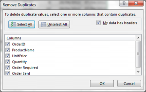
Excel 2007 and later – Remove Duplicates:
- Go to the Data tab on the ribbon
- Select Remove Duplicates.
- Check or uncheck the columns for which you want to search for duplicates.
- Click OK.
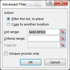
Excel 2003 and earlier (this still works on newer versions as well) – Advanced Filter:

- Go to the Data menu, choose Filter then Advanced Filter (on 2007 and later go to the Data tab and select Advanced in the Filter group).
- To output the unique values only to another cell range, select:
- Copy to another location
- In List range specify where the source data is
- In Criteria range point to the cell with your heading in
- In Copy to point to the cell with your heading in
- Check Unique records only.
- Click OK.
The unique items will then be output to a separate list. Very useful!
Using advanced filters and other filtering techniques are covered in Best STL’s Excel Intermediate course, offered London and UK wide.
At Best STL we offer Learn Excel London courses in the city and throughout the UK at a level to best suit your needs. Whether that’s an introduction, intermediate or advanced, there’s a training course to make your day run smoother.


