Categories
Excel Training

Excel Courses: Hide columns and rows in an Excel Worksheet

If you don’t want part of the Excel worksheet to be visible or when you don’t want certain data to appear in print outs, then a simple solution is to temporarily hide columns and rows.

Hide a single column:

1)    Right click on the column header of the column you want to hide (this is the grey bar along the top edge of the worksheet)

2)    Choose Hide from the menu

3)    This column will now be hidden from view
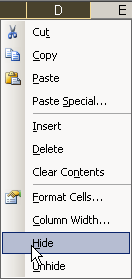
Click Hide

Hide more than one column:

1)    In the column header drag select to highlight the columns you want hidden

2)    Right click and choose Hide from the menu
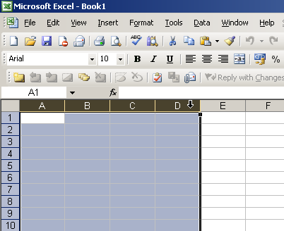
Example

Hide separate columns:

1)    Click on the fist column to be hidden

2)    Press and hold down the CTRL key

3)    While holding the CTRL key, left click on the rest of the columns you want to hide

4)    Right click and choose Hide
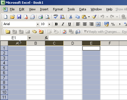
Example

Please note:- When you hide a column in an Excel worksheet, data in that column can still be used and referenced in the worksheet. 


Categories
Excel Training

Microsoft Excel 2010 – Extract Data From a Cell Using LEFT Function

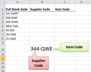
In the following example there is a column of stock codes. The numbers represent our Supplier and the letters after the hyphen (-) indicates our Item number.

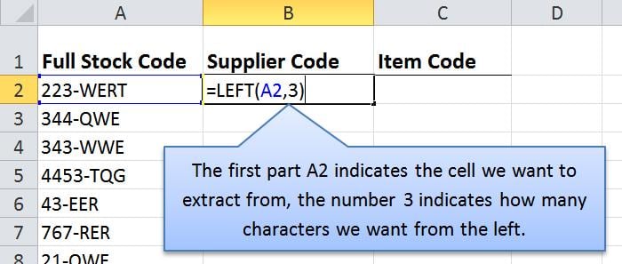
Excel Training LEFT Function

Suppose we need to extract the Supplier and Item codes and place in separate cells. If our Supplier codes were all equal length e.g. 3 numbers long, we could simply use the LEFT function.
In the Excel 2010 Training Courses here in London this is a common question.

Example:
Excel Training London Using the LEFT Function

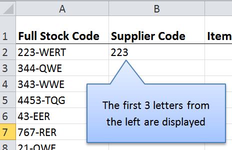
Result:
Training Excel London Results of using LEFT Function


The problem we have is that not all Supplier codes are 3 numbers in length.
We can correct this by using another Excel function word, FIND.

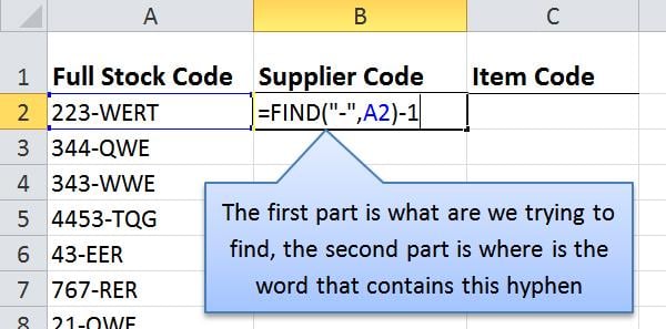
FIND function can return a number value of where a particular character appears, e.g. if we have a word “BEST-STL TRAINING” the FIND function would tell us that the hyphen is the 5th character.

We could use this inside (nested) the LEFT function – But remember we do not want to include the hyphen (-) in our final result so we need to subtract 1.

Example:
Excel 2010 Training Learn to use FIND Function

NOTE: Without subtracting 1 in the above example, it would return a value of 4

Final Code: =LEFT(A2,FIND(“-“,A2)-1)

We could repeat this for the Item code by using a combination of RIGHT, LEN and FIND nested.